Plot Inverse Probability Weights

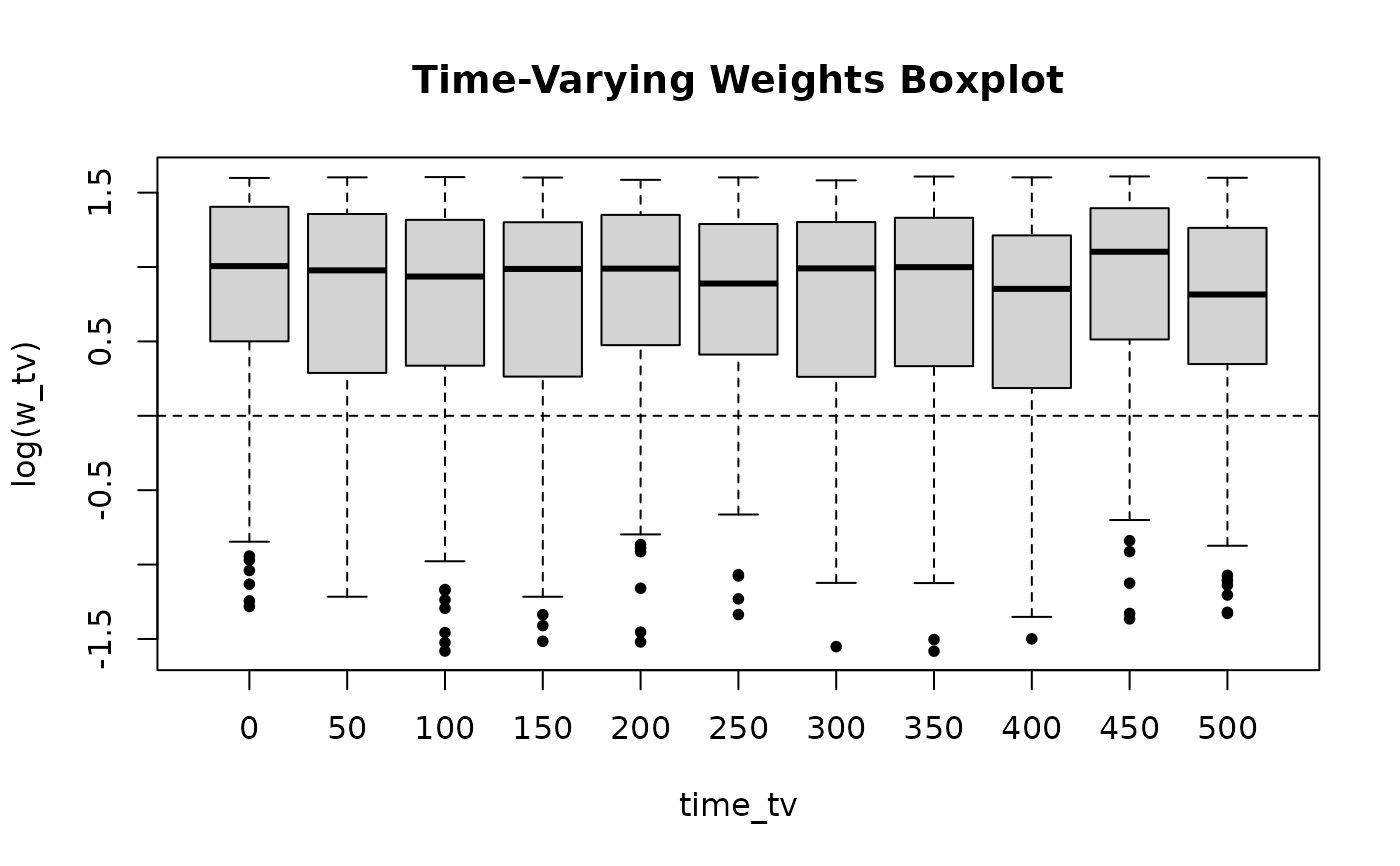
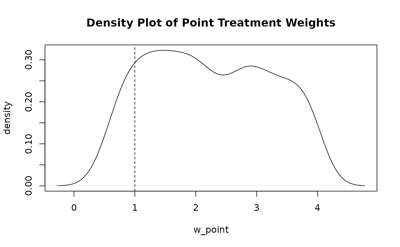
Plots the distribution of inverse probability weights. Displays a density plot for point treatment weights or boxplots across follow-up intervals for time-varying weights.

Usage

ipwplot(
  weights,
  timevar = NULL,
  binwidth = NULL,
  logscale = TRUE,
  xlab = NULL,
  ylab = NULL,
  main = "",
  ref = TRUE,
  ...
)

Arguments

weights: Numerical vector of inverse probability weights.
timevar: Optional numerical vector of follow-up time.
binwidth: Interval width for grouping follow-up time when timevar is supplied.
logscale: Logical; if TRUE, weights are plotted on a log scale. Default is TRUE.
xlab: Horizontal axis label.
ylab: Vertical axis label.
main: Main plot title.
ref: Logical; if TRUE, adds a reference line at 1 (or log(1) = 0).
...: Additional graphical parameters passed to boxplot or plot.

Author

Willem M. van der Wal willem@vanderwalresearch.com, Ronald B. Geskus rgeskus@oucru.org

Examples

# Point treatment weights density plot
set.seed(123)
w_point <- runif(500, 0.5, 4)
ipwplot(weights = w_point, logscale = FALSE, main = "Density Plot of Point Treatment Weights")


# Time-varying weights boxplot across follow-up strata
w_tv <- runif(1100, 0.2, 5)
time_tv <- rep(seq(0, 500, by = 50), each = 100)
ipwplot(weights = w_tv, timevar = time_tv, binwidth = 50, main = "Time-Varying Weights Boxplot")