Simulation study: do the weights recover known effects?

This article checks, by simulation, whether the new features of ipw do what they should: each scenario generates data in which the true causal effect is known, estimates it, and repeats this hundreds of times, in the spirit of the simulated example in the JSS paper (van der Wal & Geskus 2011).

Main findings

The new weights remove confounding when their model is correct. Naive analyses and weights from misspecified models are biased by 15% to over 200%; the new weights reduce this to 0 to 5%.
The remaining small biases (3 to 5%) are properties of inverse probability weighting, not of the implementation. Weights computed from the true model (oracle weights) have the same bias for log-normal doses, and for smooth terms and ordinal exposures the bias shrinks as the sample grows.
ipwboot() gives accurate standard errors when the weights are well behaved, where robust standard errors are 8 to 10% too large. It does not fix analyses with extreme weights: with poor overlap or long products of time-varying weights, no standard error reaches 95% coverage, and the bootstrap is then not better than the robust standard error.

How the results were produced. The study is in dev/simulation-study.R; the code below shows the essential lines of each scenario. It takes about 20 minutes on 4 cores, so this page shows saved results. To reproduce them, run Rscript dev/simulation-study.R in the package folder (seed 20261101, L’Ecuyer random numbers, 4 parallel workers), or start the simulations workflow from the GitHub Actions tab. Replications: 500 for scenarios 1 to 4, 250 for 5 and 6, 200 for the large-sample and oracle checks, 1000 for 7a and 7b, and 500 for 7c and 7d, each with 200 bootstrap samples.

Reading the tables. Bias is the mean estimate minus the truth. The MCSE (Monte Carlo standard error) shows how precisely the simulation estimates that bias: a bias within about 2 MCSE of 0 could be simulation noise. Empirical SD is the spread of the estimates; RMSE combines bias and spread.

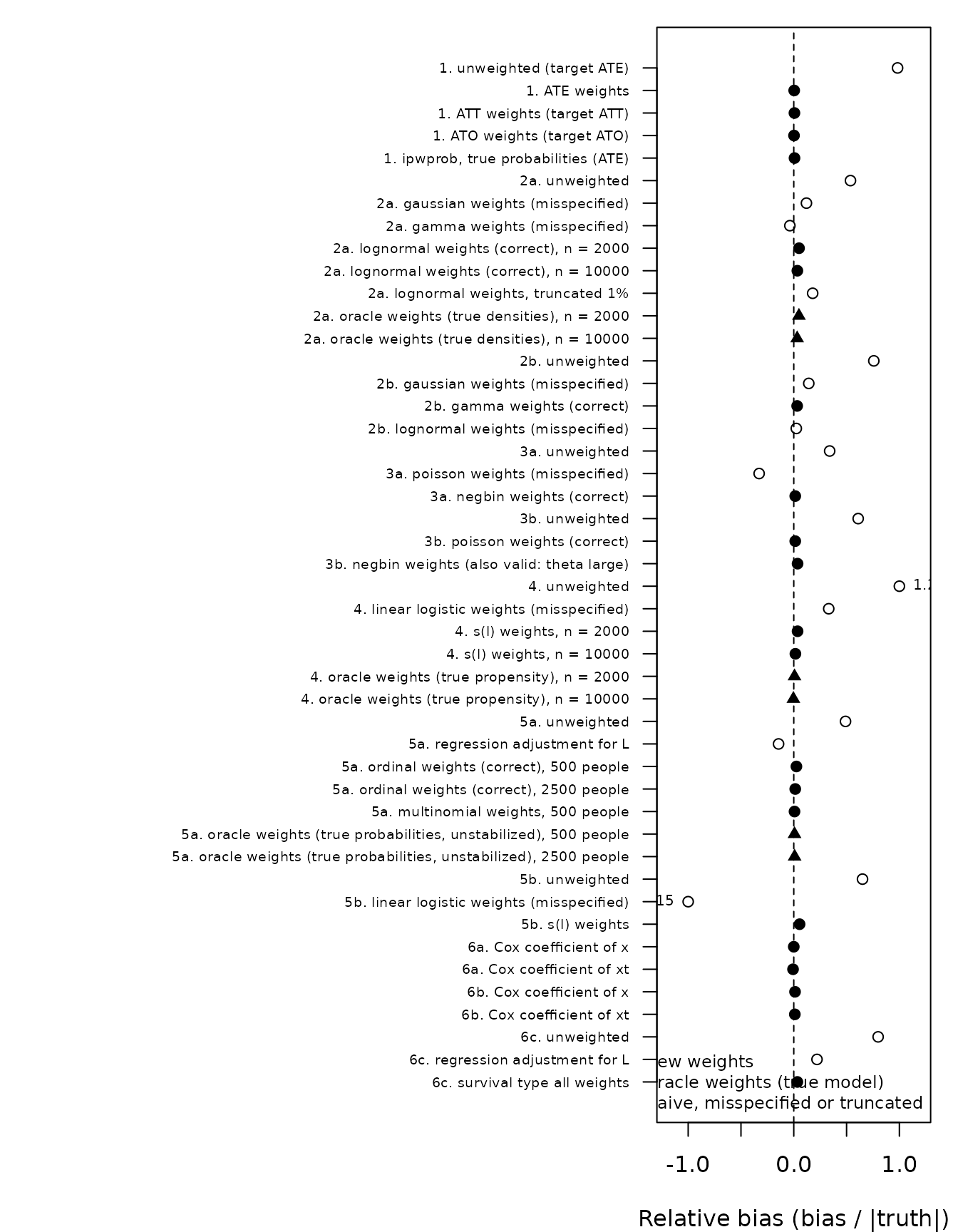
1. ATE, ATT and overlap weights, and `ipwprob()`

The effect of a binary exposure varies with the confounder l, so the three estimands differ. Their true values, from 2 million simulated people, are ATE = 1.00, ATT = 1.27 and ATO = 0.86. Each weighting scheme is compared with its own target; ipwprob() is given the true propensity scores.

d <- data.frame(l = rnorm(1000))
d$a <- rbinom(1000, 1, plogis(0.5 + 0.8 * d$l))
d$y <- d$a * (1 + d$l) + d$l + rnorm(1000)
w.att <- ipwpoint(exposure = a, family = "binomial", link = "logit",
                  denominator = ~ l, data = d, estimand = "ATT")$ipw.weights
coef(lm(y ~ a, data = d, weights = w.att))["a"]

Method	Truth	Mean estimate	Bias	MCSE of bias	Empirical SD	RMSE	Replications
unweighted (target ATE)	0.999	1.981	0.982	0.005	0.112	0.988	500
ATE weights	0.999	1.003	0.004	0.004	0.080	0.080	500
ATT weights (target ATT)	1.275	1.283	0.008	0.004	0.099	0.099	500
ATO weights (target ATO)	0.861	0.863	0.002	0.003	0.078	0.078	500
ipwprob, true probabilities (ATE)	0.999	1.006	0.007	0.006	0.139	0.139	500

All weighted estimates are within 1% of their own estimand; the unweighted difference is twice the ATE.

2. Skewed continuous exposures: gaussian, gamma or log-normal

One unit of dose raises the outcome by 1. In 2a the dose is log-normal given l, in 2b gamma. In 2a the true densities are known, so oracle weights (the true marginal density over the true conditional density) show what weighting can achieve without any estimation error; they are also computed for a 5 times larger sample.

d <- data.frame(l = rnorm(2000))
d$dose <- exp(0.5 + 0.5 * d$l + rnorm(2000, 0, 0.6))   # 2b: rgamma(2000, 3, 3 / exp(0.5 + 0.3 * d$l))
d$y <- d$dose + 2 * d$l + rnorm(2000)
w.ln <- ipwpoint(exposure = dose, family = "lognormal", numerator = ~ 1,
                 denominator = ~ l, data = d)$ipw.weights
oracle <- dlnorm(d$dose, 0.5, sqrt(0.61)) / dlnorm(d$dose, 0.5 + 0.5 * d$l, 0.6)

Method	Truth	Mean estimate	Bias	MCSE of bias	Empirical SD	RMSE	Replications
unweighted	1	1.537	0.537	0.002	0.041	0.538	500
gaussian weights (misspecified)	1	1.120	0.120	0.015	0.344	0.363	493
gamma weights (misspecified)	1	0.963	-0.037	0.008	0.177	0.181	500
lognormal weights (correct), n = 2000	1	1.050	0.050	0.004	0.096	0.108	500
lognormal weights (correct), n = 10000	1	1.034	0.034	0.005	0.065	0.073	200
lognormal weights, truncated 1%	1	1.179	0.179	0.002	0.038	0.183	500
oracle weights (true densities), n = 2000	1	1.049	0.049	0.005	0.104	0.115	500
oracle weights (true densities), n = 10000	1	1.032	0.032	0.005	0.067	0.074	200

Method	Truth	Mean estimate	Bias	MCSE of bias	Empirical SD	RMSE	Replications
unweighted	1	1.758	0.758	0.002	0.040	0.759	500
gaussian weights (misspecified)	1	1.142	0.142	0.004	0.079	0.162	500
gamma weights (correct)	1	1.032	0.032	0.005	0.111	0.115	500
lognormal weights (misspecified)	1	1.024	0.024	0.010	0.220	0.221	500

The correct family removes most of the confounding (unweighted bias 54% and 76%). The 3 to 5% that remains is the same for oracle weights (5.0% vs 4.9% at n = 2000, 3.4% vs 3.2% at n = 10000), so it does not come from estimating the model: it is the finite-sample bias of weighting with densities of a skewed exposure, whose density ratios have a heavy tail, and it shrinks slowly as the sample grows. The gaussian model is clearly worse, and in 7 of 500 replications gave infinite weights, which ipwpoint() refuses. A misspecified skewed family (gamma for log-normal data or the reverse) has a small bias but up to twice the spread. Truncation reduces the spread a lot but adds bias.

3. Count exposures: Poisson or negative binomial

Each extra unit of a count exposure raises the outcome by 0.5. In 3a the counts are overdispersed (negative binomial); in 3b they are Poisson.

d <- data.frame(l = rnorm(1000))
d$v <- rnbinom(1000, size = 2, mu = exp(0.5 + 0.4 * d$l))   # 3b: rpois(1000, exp(0.5 + 0.4 * d$l))
d$y <- 0.5 * d$v + d$l + rnorm(1000)
w.nb <- ipwpoint(exposure = v, family = "negbin", numerator = ~ 1,
                 denominator = ~ l, data = d)$ipw.weights

Method	Truth	Mean estimate	Bias	MCSE of bias	Empirical SD	RMSE	Replications
unweighted	0.5	0.670	0.170	0.001	0.022	0.171	500
poisson weights (misspecified)	0.5	0.336	-0.164	0.003	0.068	0.178	500
negbin weights (correct)	0.5	0.507	0.007	0.002	0.035	0.035	500
unweighted	0.5	0.805	0.305	0.001	0.028	0.307	500
poisson weights (correct)	0.5	0.507	0.007	0.003	0.062	0.063	500
negbin weights (also valid: theta large)	0.5	0.518	0.018	0.003	0.064	0.066	500

With the correct model, both families are within 1.5% of the truth. The Poisson model applied to overdispersed counts over-corrects as strongly as the unweighted analysis under-corrects. The negative binomial model remains usable for Poisson data (bias 3.6%), so it is the safer choice when in doubt.

4. Curved propensity: smooth terms with mgcv

The probability of exposure depends on l through a sine curve; the true effect is 2. Oracle weights use the true propensity.

d <- data.frame(l = runif(2000, -2, 2))
d$a <- rbinom(2000, 1, plogis(2 * sin(1.5 * d$l)))
d$y <- 2 * d$a + 3 * sin(1.5 * d$l) + rnorm(2000)
w.gam <- ipwpoint(exposure = a, family = "binomial", link = "logit",
                  numerator = ~ 1, denominator = ~ s(l), data = d)$ipw.weights

Method	Truth	Mean estimate	Bias	MCSE of bias	Empirical SD	RMSE	Replications
unweighted	2	4.553	2.553	0.004	0.090	2.554	500
linear logistic weights (misspecified)	2	2.662	0.662	0.004	0.079	0.667	500
s(l) weights, n = 2000	2	2.072	0.072	0.003	0.062	0.095	500
s(l) weights, n = 10000	2	2.031	0.031	0.002	0.026	0.040	200
oracle weights (true propensity), n = 2000	2	2.014	0.014	0.007	0.148	0.149	500
oracle weights (true propensity), n = 10000	2	1.993	-0.007	0.005	0.065	0.066	200

A straight-line logistic model leaves a quarter of the confounding bias. With s(l) the bias is 3.6% at n = 2000 and 1.5% at n = 10000: it halves as the sample grows five-fold, as expected for a smoothing estimate that approaches the true curve. Oracle weights are unbiased, which confirms that the remaining bias comes from estimating the curve.

5. Time-varying exposure, `type = "all"`

5a. Ordinal dose

A dose level (0, 1, 2) is chosen at each of 4 visits from a proportional-odds model given the confounder L and the previous dose. L is affected by the previous dose and by an unmeasured U that also affects the outcome; the outcome rises by 1 per unit of cumulative dose. This is the situation in the JSS paper where ordinary adjustment fails.

for (t in 1:4) {
  l <- U + 0.4 * prev + rnorm(n, 0, 0.5)
  dose <- findInterval(0.8 * l + 0.6 * prev + rlogis(n), c(0, 1.5))   # 0, 1, 2
  prev <- dose
}
y <- cumulative.dose + 2 * U + rnorm(n)
w <- ipwtm(exposure = dose, family = "ordinal", link = "logit",
           numerator = ~ dose.lag, denominator = ~ dose.lag + l,
           id = id, timevar = time, type = "all", data = long)
# weight at the last visit, then lm(y ~ cumulative.dose, weights = ...)

Method	Truth	Mean estimate	Bias	MCSE of bias	Empirical SD	RMSE	Replications
unweighted	1	1.490	0.490	0.002	0.034	0.491	250
regression adjustment for L	1	0.856	-0.144	0.002	0.029	0.147	250
ordinal weights (correct), 500 people	1	1.025	0.025	0.008	0.122	0.124	250
ordinal weights (correct), 2500 people	1	1.014	0.014	0.005	0.073	0.074	200
multinomial weights, 500 people	1	1.007	0.007	0.008	0.133	0.133	250
oracle weights (true probabilities, unstabilized), 500 people	1	1.007	0.007	0.010	0.152	0.152	250
oracle weights (true probabilities, unstabilized), 2500 people	1	1.008	0.008	0.006	0.083	0.084	200

Both naive analyses are biased (+49% and -14%). Ordinal and multinomial weights recover the effect; the 2.5% bias of the ordinal weights at 500 people falls to 1.4% at 2500, and oracle weights are within 1%.

5b. Smooth terms in `ipwtm()`

A binary exposure is chosen at each visit with a curved effect of L (logit = -0.3 + 2 sin(1.5 L) + 0.6 × previous exposure), in the same design.

w <- ipwtm(exposure = a, family = "binomial", link = "logit", numerator = ~ a.lag,
           denominator = ~ a.lag + s(l), id = id, timevar = time, type = "all", data = long)

Method	Truth	Mean estimate	Bias	MCSE of bias	Empirical SD	RMSE	Replications
unweighted	1	1.651	0.651	0.004	0.061	0.654	250
linear logistic weights (misspecified)	1	-0.152	-1.152	0.033	0.526	1.266	250
s(l) weights	1	1.055	0.055	0.015	0.243	0.249	250

Here a straight-line model is worse than no weighting at all: its weights turn the effect of +1 into a negative estimate. With s(l) the bias is 5.5%.

6. Recurrent exposure events, `family = "survival"`, `type = "all"`

6a and 6b. Weights against the true weights

Exposure events (for example new prescriptions) happen repeatedly with a known proportional hazard: baseline 2 per unit time, log hazard ratio 0.5 for a fixed covariate x and -1 for a time-varying covariate xt. Because the true hazard is known, the true weights are known too. In 6a all people share a grid of 10 intervals (as in haartdat); in 6b the events happen in continuous time, xt changes at different times for each person, and each event ends an interval (start-stop data cut at events, as in Graffeo et al. 2018).

w <- ipwtm(exposure = expo, family = "survival", denominator = ~ x + xt,
           id = id, tstart = tstart, timevar = fuptime, type = "all", data = d)
coef(w$den.mod)
median(abs(log(w$ipw.weights / true.weights)))

Method	Truth	Mean estimate	Bias	MCSE of bias	Empirical SD	RMSE	Replications
Cox coefficient of x	0.5	0.500	0.000	0.006	0.088	0.088	250
Cox coefficient of xt	-1.0	-1.007	-0.007	0.007	0.118	0.118	250
median \|log(estimated / true weight)\|	0.0	0.074	0.074	0.001	0.022	0.077	250

Method	Truth	Mean estimate	Bias	MCSE of bias	Empirical SD	RMSE	Replications
Cox coefficient of x	0.5	0.506	0.006	0.005	0.084	0.084	250
Cox coefficient of xt	-1.0	-0.990	0.010	0.007	0.104	0.104	250
median \|log(estimated / true weight)\|	0.0	0.090	0.090	0.001	0.022	0.092	250

The Cox coefficients are unbiased in both designs, and the estimated weights are typically within 7 to 9% of the true weights, which is the estimation noise of the baseline hazard.

6c. Causal effect of the number of exposure events

Exposure events happen in continuous time with hazard 1.5 exp(0.6 L). L is updated at 4 visits, is lowered by earlier events (as treatment raising CD4 lowers the need for more) and depends on an unmeasured U that also affects the outcome. The outcome rises by 1 per event.

w <- ipwtm(exposure = expo, family = "survival", numerator = ~ 1, denominator = ~ l,
           id = id, tstart = tstart, timevar = fuptime, type = "all", data = d)
# weight at each person's last row, then lm(y ~ number.of.events, weights = ...)

Method	Truth	Mean estimate	Bias	MCSE of bias	Empirical SD	RMSE	Replications
unweighted	1	1.799	0.799	0.004	0.060	0.801	250
regression adjustment for L	1	1.220	0.220	0.003	0.047	0.224	250
survival type all weights	1	1.034	0.034	0.012	0.193	0.196	250

The weights reduce the bias from 80% (unweighted) and 22% (adjustment for L) to 3.4%. The method of Graffeo et al. uses, for an interval ending in an event, the probability of an event during that interval; this simulation shows that the approximation works for estimating a causal effect.

7. Standard errors: `ipwboot()`, robust and naive

Each table shows the mean estimated standard error divided by the actual spread of the estimates (1 is ideal) and the coverage of 95% confidence intervals.

7a and 7b. Linear MSM for a binary exposure

True effect 10, n = 500, stabilized weights. In 7a, exposure probabilities are mostly between 0.1 and 0.9 (good overlap); 7b is the simulated example of the JSS paper, where many people are almost certain to be exposed or unexposed.

msm.effect <- function(dd) {
  w <- ipwpoint(exposure = a, family = "binomial", link = "logit", numerator = ~ 1,
                denominator = ~ l, data = dd)$ipw.weights
  coef(lm(y ~ a, data = dd, weights = w))["a"]
}
ipwboot(d, msm.effect, R = 200)

Method	Mean estimate	Mean SE	Empirical SD	SE / empirical SD	Coverage of 95% CI	MCSE of coverage	Replications
ipwboot, percentile CI	9.981	0.492	0.487	1.011	0.936	0.008	1000
ipwboot SE, Wald CI	9.981	0.492	0.487	1.011	0.947	0.007	1000
robust SE (svyglm), Wald CI	9.981	0.536	0.487	1.101	0.967	0.006	1000

Method	Mean estimate	Mean SE	Empirical SD	SE / empirical SD	Coverage of 95% CI	MCSE of coverage	Replications
ipwboot, percentile CI	11.019	1.110	1.787	0.621	0.560	0.016	1000
ipwboot SE, Wald CI	11.019	1.110	1.787	0.621	0.585	0.016	1000
robust SE (svyglm), Wald CI	11.019	1.113	1.787	0.623	0.591	0.016	1000

With good overlap the bootstrap standard error is accurate (ratio 1.01, Wald coverage 94.7%), while the robust standard error is 10% too large (coverage 96.7%), in line with Austin (2016); percentile intervals cover slightly less than 95%. In the JSS example the estimate itself is biased (11.0 instead of 10) and all standard errors are 38% too small, so coverage is below 60% whatever method is used.

7c. Weighted Cox MSM

Austin (2016) studied weighted Cox models. Here event times are exponential with hazard 0.1 exp(-0.7 a + 0.8 l), censored at 5; n = 1000. The true marginal log hazard ratio, -0.624, is computed from both potential outcomes of 200,000 people (it differs from -0.7 because hazard ratios are not collapsible).

Method	Mean estimate	Mean SE	Empirical SD	SE / empirical SD	Coverage of 95% CI	MCSE of coverage	Replications
naive SE (coxph), Wald CI	-0.61	0.117	0.113	1.037	0.952	0.010	500
robust SE (coxph), Wald CI	-0.61	0.122	0.113	1.078	0.960	0.009	500
ipwboot SE, Wald CI	-0.61	0.110	0.113	0.974	0.936	0.011	500
ipwboot, percentile CI	-0.61	0.110	0.113	0.974	0.934	0.011	500

All three standard errors are close to the truth here. The robust standard error is again too large (+8%); the naive one (+4%) and the bootstrap (-3%) are within simulation noise of 1. With stabilized weights and good overlap, the bootstrap therefore brings no clear gain over the naive standard error in this setting.

7d. Time-varying exposure, bootstrap by person

The design of scenario 5 with a binary exposure; ipwboot(id = id) resamples people with all their visits.

ipwboot(long, tv.effect, id = id, R = 200)

Method	Mean estimate	Mean SE	Empirical SD	SE / empirical SD	Coverage of 95% CI	MCSE of coverage	Replications
ipwboot (id), percentile CI	1.033	0.146	0.222	0.658	0.778	0.019	500
ipwboot (id) SE, Wald CI	1.033	0.146	0.222	0.658	0.792	0.018	500
robust SE (svyglm), Wald CI	1.033	0.163	0.222	0.737	0.838	0.016	500

Neither method is adequate here: the bootstrap standard error is 34% too small and the robust one 26% too small, with coverage of 79% and 84%. The weights are products over 4 visits, so a few people get very large weights and the estimate has a heavy-tailed distribution that 500 people do not represent well, the same problem as in 7b. Truncation, a larger sample or a better-balanced design would be needed; the bootstrap does not repair it.

Conclusions

The simulations support the new models: with the correct model, each of them removes nearly all confounding, and the small biases that remain are either shared by weights from the true model or shrink with the sample size. They support ipwboot() for analyses with well-behaved weights, where it gives accurate standard errors and robust standard errors are conservative. They also show its limit: when weights are extreme (poor overlap, long products of time-varying weights), no standard error is reliable, and the first step is to examine the weights (summary(), ipwplot()) and consider overlap weights, truncation or a different model.

References

Austin PC (2016). Variance estimation when using inverse probability of treatment weighting (IPTW) with survival analysis. Statistics in Medicine 35, 5642-5655.
Graffeo N, Latouche A, Geskus RB, Chevret S (2018). Modeling time-varying exposure using inverse probability of treatment weights. Biometrical Journal 60, 323-332.
Li F, Morgan KL, Zaslavsky AM (2018). Balancing covariates via propensity score weighting. Journal of the American Statistical Association 113, 390-400.
van der Wal WM, Geskus RB (2011). ipw: An R package for inverse probability weighting. Journal of Statistical Software 43(13), 1-23.

1. ATE, ATT and overlap weights, and ipwprob()