Estimates inverse probability weights to fit marginal structural models in a
point treatment situation. Exposure can be binomial, multinomial, ordinal,
a count (Poisson or negative binomial) or continuous (gaussian, gamma or
log-normal). Both stabilized and unstabilized weights can be estimated, and
for a binomial exposure also weights for the effect in the treated (ATT) and
overlap weights (ATO). Formulas may contain smooth terms such as s(x),
which are then fitted as generalized additive models with mgcv.
Usage
ipwpoint(
  exposure,
  family,
  link = NULL,
  numerator = NULL,
  denominator,
  data,
  trunc = NULL,
  estimand = c("ATE", "ATT", "ATO"),
  ...
)
Arguments
- exposure
Name of the exposure column in
data(unquoted or as a string). Binomial exposure variables should be coded as 0/1.- family
Model family for exposure:
"binomial","multinomial","ordinal","gaussian","poisson","negbin"(negative binomial, fitted withMASS::glm.nb),"gamma"(gamma GLM with log link) or"lognormal"(normal model for the log of the exposure). Count exposures must be non-negative integers; gamma and log-normal exposures must be positive.- link
Link function for binomial (
"logit","probit","cauchit","log","cloglog") or ordinal ("logit","probit","cauchit","cloglog"). Ignored for multinomial and gaussian.- numerator
Formula specifying the right-hand side of the numerator model. If
NULL, unstabilized weights (numerator = 1) are calculated. Required for the continuous families ("gaussian","gamma","lognormal"); must beNULLwhenestimandis"ATT"or"ATO".- denominator
Formula specifying the right-hand side of the denominator model. Smooth terms (
s(),te(),ti(),t2()) are allowed for the binomial, gaussian and poisson families; the model is then fitted withmgcv::gam.- data
Data frame containing exposure and model covariates.
- trunc
Optional truncation percentile between 0 and 0.5 (e.g., 0.01 for 1st/99th percentiles).
- estimand
Target estimand for a binomial exposure:
"ATE"(default; inverse probability weights),"ATT"(treated get weight 1, untreated \(p/(1-p)\)) or"ATO"(overlap weights: treated \(1-p\), untreated \(p\)), where \(p\) is the fitted probability of exposure from the denominator model.- ...
Additional arguments passed to model fitting functions (
glm,multinom,polr,glm.nb,gam).
Value
A list of class "ipwpoint" containing:
- ipw.weights
Numeric vector of inverse probability weights.
- weights.trunc
Numeric vector of truncated weights (if
truncis specified).- call
The original function call.
- num.mod
Numerator model object (if
numeratoris specified).- den.mod
Denominator model object.
Details
Standard errors: ipwpoint only estimates the weights. Standard errors
for the marginal structural model have to be obtained when that model is fitted.
Robust (sandwich) standard errors, for example from svyglm() in the survey
package as in Van der Wal and Geskus (2011), treat the weights as known and tend to
be conservative (too large). Austin (2016) compared naive, robust and bootstrap
standard errors in simulations and recommends the bootstrap, in which the weights
are re-estimated in each bootstrap sample. This takes the uncertainty in the
estimated weights into account; see the bootstrap example below, or use
ipwboot, which does this for you. About 200 bootstrap samples are
usually enough to estimate a standard error. In the package's simulation study
(article "Simulation study" on the package website), the bootstrap standard
error was accurate for a point treatment with good overlap, while robust
standard errors were about 10% too large. When some weights are extreme
(poor overlap), no standard error was reliable, the bootstrap included. Check
the weights first with summary() and ipwplot, and consider
truncation (trunc) or overlap weights (estimand = "ATO").
References
Cole, S.R. & Hernán, M.A. (2008). Constructing inverse probability weights for marginal structural models. American Journal of Epidemiology, 168(6), 656-664.
Robins, J.M., Hernán, M.A. & Brumback, B.A. (2000). Marginal structural models and causal inference in epidemiology. Epidemiology, 11, 550-560.
Van der Wal W.M. & Geskus R.B. (2011). ipw: An R Package for Inverse Probability Weighting. Journal of Statistical Software, 43(13), 1-23. doi:10.18637/jss.v043.i13 .
Austin, P.C. (2016). Variance estimation when using inverse probability of treatment weighting (IPTW) with survival analysis. Statistics in Medicine, 35, 5642-5655. doi:10.1002/sim.7084 .
Author
Willem M. van der Wal willem@vanderwalresearch.com, Ronald B. Geskus rgeskus@oucru.org, Hung Thai Tran hungtt@oucru.org
Examples
# Simulate data with continuous confounder and outcome, binomial exposure.
# Marginal causal effect of exposure on outcome: 10.
set.seed(16)
n <- 1000
simdat <- data.frame(l = rnorm(n, 10, 5))
a.lin <- simdat$l - 10
pa <- exp(a.lin)/(1 + exp(a.lin))
simdat$a <- rbinom(n, 1, prob = pa)
simdat$y <- 10*simdat$a + 0.5*simdat$l + rnorm(n, -10, 5)
simdat[1:5,]
#> l a y
#> 1 12.382067 1 6.635898
#> 2 9.373100 0 -11.722042
#> 3 15.481081 1 11.501612
#> 4 2.778855 0 -9.464074
#> 5 15.739146 1 15.085261
# Estimate ipw weights
temp <- ipwpoint(
exposure = a,
family = "binomial",
link = "logit",
numerator = ~ 1,
denominator = ~ l,
data = simdat)
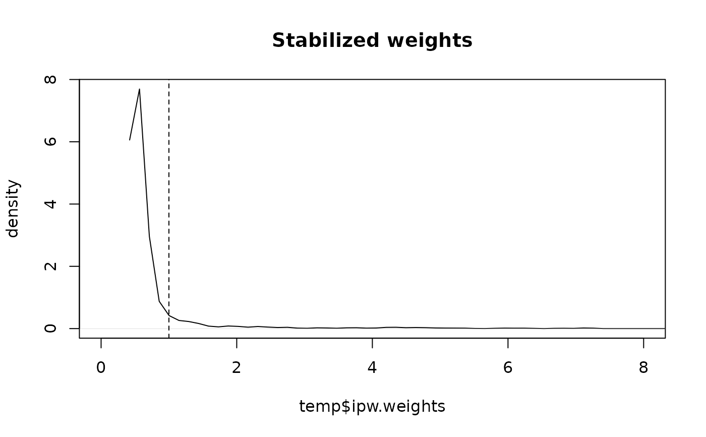
summary(temp$ipw.weights)
#> Min. 1st Qu. Median Mean 3rd Qu. Max.
#> 0.4810 0.5127 0.5285 0.9095 0.6318 74.6994
# Plot inverse probability weights
ipwplot(weights = temp$ipw.weights, logscale = FALSE,
main = "Stabilized weights", xlim = c(0, 8))
 # Examine numerator and denominator models
summary(temp$num.mod)
#>
#> Call:
#> (function (formula, family = gaussian, data, weights, subset,
#> na.action, start = NULL, etastart, mustart, offset, control = list(...),
#> model = TRUE, method = "glm.fit", x = FALSE, y = TRUE, singular.ok = TRUE,
#> contrasts = NULL, ...)
#> {
#> cal <- match.call()
#> if (is.character(family))
#> family <- get(family, mode = "function", envir = parent.frame())
#> if (is.function(family))
#> family <- family()
#> if (is.null(family$family)) {
#> print(family)
#> stop("'family' not recognized")
#> }
#> if (missing(data))
#> data <- environment(formula)
#> mf <- match.call(expand.dots = FALSE)
#> m <- match(c("formula", "data", "subset", "weights", "na.action",
#> "etastart", "mustart", "offset"), names(mf), 0L)
#> mf <- mf[c(1L, m)]
#> mf$drop.unused.levels <- TRUE
#> mf[[1L]] <- quote(stats::model.frame)
#> mf <- eval(mf, parent.frame())
#> if (identical(method, "model.frame"))
#> return(mf)
#> if (!is.character(method) && !is.function(method))
#> stop("invalid 'method' argument")
#> if (identical(method, "glm.fit"))
#> control <- do.call("glm.control", control)
#> mt <- attr(mf, "terms")
#> Y <- model.response(mf, "any")
#> if (length(dim(Y)) == 1L) {
#> nm <- rownames(Y)
#> dim(Y) <- NULL
#> if (!is.null(nm))
#> names(Y) <- nm
#> }
#> X <- if (!is.empty.model(mt))
#> model.matrix(mt, mf, contrasts)
#> else matrix(, NROW(Y), 0L)
#> weights <- as.vector(model.weights(mf))
#> if (!is.null(weights) && !is.numeric(weights))
#> stop("'weights' must be a numeric vector")
#> if (!is.null(weights) && any(weights < 0))
#> stop("negative weights not allowed")
#> offset <- as.vector(model.offset(mf))
#> if (!is.null(offset)) {
#> if (length(offset) != NROW(Y))
#> stop(gettextf("number of offsets is %d should equal %d (number of observations)",
#> length(offset), NROW(Y)), domain = NA)
#> }
#> mustart <- model.extract(mf, "mustart")
#> etastart <- model.extract(mf, "etastart")
#> fit <- eval(call(if (is.function(method)) "method" else method,
#> x = X, y = Y, weights = weights, start = start, etastart = etastart,
#> mustart = mustart, offset = offset, family = family,
#> control = control, intercept = attr(mt, "intercept") >
#> 0L, singular.ok = singular.ok))
#> if (length(offset) && attr(mt, "intercept") > 0L) {
#> fit2 <- eval(call(if (is.function(method)) "method" else method,
#> x = X[, "(Intercept)", drop = FALSE], y = Y, mustart = fit$fitted.values,
#> weights = weights, offset = offset, family = family,
#> control = control, intercept = TRUE))
#> if (!fit2$converged)
#> warning("fitting to calculate the null deviance did not converge -- increase 'maxit'?")
#> fit$null.deviance <- fit2$deviance
#> }
#> if (model)
#> fit$model <- mf
#> fit$na.action <- attr(mf, "na.action")
#> if (x)
#> fit$x <- X
#> if (!y)
#> fit$y <- NULL
#> structure(c(fit, list(call = cal, formula = formula, terms = mt,
#> data = data, offset = offset, control = control, method = method,
#> contrasts = attr(X, "contrasts"), xlevels = .getXlevels(mt,
#> mf))), class = c(fit$class, c("glm", "lm")))
#> })(formula = a ~ 1, family = binomial(link = "logit"), data = simdat,
#> na.action = function (object, ...)
#> UseMethod("na.fail"))
#>
#> Coefficients:
#> Estimate Std. Error z value Pr(>|z|)
#> (Intercept) 0.07604 0.06329 1.201 0.23
#>
#> (Dispersion parameter for binomial family taken to be 1)
#>
#> Null deviance: 1384.9 on 999 degrees of freedom
#> Residual deviance: 1384.9 on 999 degrees of freedom
#> AIC: 1386.9
#>
#> Number of Fisher Scoring iterations: 3
#>
summary(temp$den.mod)
#>
#> Call:
#> (function (formula, family = gaussian, data, weights, subset,
#> na.action, start = NULL, etastart, mustart, offset, control = list(...),
#> model = TRUE, method = "glm.fit", x = FALSE, y = TRUE, singular.ok = TRUE,
#> contrasts = NULL, ...)
#> {
#> cal <- match.call()
#> if (is.character(family))
#> family <- get(family, mode = "function", envir = parent.frame())
#> if (is.function(family))
#> family <- family()
#> if (is.null(family$family)) {
#> print(family)
#> stop("'family' not recognized")
#> }
#> if (missing(data))
#> data <- environment(formula)
#> mf <- match.call(expand.dots = FALSE)
#> m <- match(c("formula", "data", "subset", "weights", "na.action",
#> "etastart", "mustart", "offset"), names(mf), 0L)
#> mf <- mf[c(1L, m)]
#> mf$drop.unused.levels <- TRUE
#> mf[[1L]] <- quote(stats::model.frame)
#> mf <- eval(mf, parent.frame())
#> if (identical(method, "model.frame"))
#> return(mf)
#> if (!is.character(method) && !is.function(method))
#> stop("invalid 'method' argument")
#> if (identical(method, "glm.fit"))
#> control <- do.call("glm.control", control)
#> mt <- attr(mf, "terms")
#> Y <- model.response(mf, "any")
#> if (length(dim(Y)) == 1L) {
#> nm <- rownames(Y)
#> dim(Y) <- NULL
#> if (!is.null(nm))
#> names(Y) <- nm
#> }
#> X <- if (!is.empty.model(mt))
#> model.matrix(mt, mf, contrasts)
#> else matrix(, NROW(Y), 0L)
#> weights <- as.vector(model.weights(mf))
#> if (!is.null(weights) && !is.numeric(weights))
#> stop("'weights' must be a numeric vector")
#> if (!is.null(weights) && any(weights < 0))
#> stop("negative weights not allowed")
#> offset <- as.vector(model.offset(mf))
#> if (!is.null(offset)) {
#> if (length(offset) != NROW(Y))
#> stop(gettextf("number of offsets is %d should equal %d (number of observations)",
#> length(offset), NROW(Y)), domain = NA)
#> }
#> mustart <- model.extract(mf, "mustart")
#> etastart <- model.extract(mf, "etastart")
#> fit <- eval(call(if (is.function(method)) "method" else method,
#> x = X, y = Y, weights = weights, start = start, etastart = etastart,
#> mustart = mustart, offset = offset, family = family,
#> control = control, intercept = attr(mt, "intercept") >
#> 0L, singular.ok = singular.ok))
#> if (length(offset) && attr(mt, "intercept") > 0L) {
#> fit2 <- eval(call(if (is.function(method)) "method" else method,
#> x = X[, "(Intercept)", drop = FALSE], y = Y, mustart = fit$fitted.values,
#> weights = weights, offset = offset, family = family,
#> control = control, intercept = TRUE))
#> if (!fit2$converged)
#> warning("fitting to calculate the null deviance did not converge -- increase 'maxit'?")
#> fit$null.deviance <- fit2$deviance
#> }
#> if (model)
#> fit$model <- mf
#> fit$na.action <- attr(mf, "na.action")
#> if (x)
#> fit$x <- X
#> if (!y)
#> fit$y <- NULL
#> structure(c(fit, list(call = cal, formula = formula, terms = mt,
#> data = data, offset = offset, control = control, method = method,
#> contrasts = attr(X, "contrasts"), xlevels = .getXlevels(mt,
#> mf))), class = c(fit$class, c("glm", "lm")))
#> })(formula = a ~ l, family = binomial(link = "logit"), data = simdat,
#> na.action = function (object, ...)
#> UseMethod("na.fail"))
#>
#> Coefficients:
#> Estimate Std. Error z value Pr(>|z|)
#> (Intercept) -9.69809 0.66066 -14.68 <2e-16 ***
#> l 0.97272 0.06525 14.91 <2e-16 ***
#> ---
#> Signif. codes: 0 ‘***’ 0.001 ‘**’ 0.01 ‘*’ 0.05 ‘.’ 0.1 ‘ ’ 1
#>
#> (Dispersion parameter for binomial family taken to be 1)
#>
#> Null deviance: 1384.85 on 999 degrees of freedom
#> Residual deviance: 496.86 on 998 degrees of freedom
#> AIC: 500.86
#>
#> Number of Fisher Scoring iterations: 7
#>
# Paste inverse probability weights
simdat$sw <- temp$ipw.weights
# Marginal structural model for the causal effect of a on y
# corrected for confounding by l using inverse probability weighting
if (requireNamespace("survey", quietly = TRUE)) {
library(survey)
msm <- svyglm(y ~ a,
design = svydesign(~1, weights = ~temp$ipw.weights,
data = simdat))
summary(msm)
}
#> Loading required package: grid
#> Loading required package: Matrix
#> Loading required package: survival
#>
#> Attaching package: ‘survey’
#> The following object is masked from ‘package:graphics’:
#>
#> dotchart
#>
#> Call:
#> svyglm(formula = y ~ a, design = svydesign(~1, weights = ~temp$ipw.weights,
#> data = simdat))
#>
#> Survey design:
#> svydesign(~1, weights = ~temp$ipw.weights, data = simdat)
#>
#> Coefficients:
#> Estimate Std. Error t value Pr(>|t|)
#> (Intercept) -4.375 1.142 -3.832 0.000135 ***
#> a 10.647 1.190 8.948 < 2e-16 ***
#> ---
#> Signif. codes: 0 ‘***’ 0.001 ‘**’ 0.01 ‘*’ 0.05 ‘.’ 0.1 ‘ ’ 1
#>
#> (Dispersion parameter for gaussian family taken to be 29.58889)
#>
#> Number of Fisher Scoring iterations: 2
#>
# Bootstrap standard error and percentile confidence interval for the MSM.
# The robust standard error from svyglm() treats the weights as known and
# tends to be conservative. Austin (2016) recommends the bootstrap, with the
# weights re-estimated in each bootstrap sample: each bootstrap sample below
# re-fits ipwpoint() and the MSM. (A weighted lm() gives the same point
# estimate as svyglm() and is faster.)
if (requireNamespace("boot", quietly = TRUE)) {
boot.fun <- function(data, index) {
d <- data[index, ]
w <- ipwpoint(
exposure = a,
family = "binomial",
link = "logit",
numerator = ~ 1,
denominator = ~ l,
data = d)
d$sw <- w$ipw.weights
coef(lm(y ~ a, data = d, weights = sw))["a"]
}
set.seed(1)
bootres <- boot::boot(data = simdat, statistic = boot.fun, R = 200)
print(bootres)
# bootstrap standard error
print(sd(bootres$t[, 1]))
# percentile 95 percent confidence interval
print(boot::boot.ci(bootres, type = "perc"))
}
#>
#> ORDINARY NONPARAMETRIC BOOTSTRAP
#>
#>
#> Call:
#> boot::boot(data = simdat, statistic = boot.fun, R = 200)
#>
#>
#> Bootstrap Statistics :
#> original bias std. error
#> t1* 10.64661 0.2146065 1.115705
#> [1] 1.115705
#> BOOTSTRAP CONFIDENCE INTERVAL CALCULATIONS
#> Based on 200 bootstrap replicates
#>
#> CALL :
#> boot::boot.ci(boot.out = bootres, type = "perc")
#>
#> Intervals :
#> Level Percentile
#> 95% ( 8.43, 12.79 )
#> Calculations and Intervals on Original Scale
#> Some percentile intervals may be unstable